A simple, yet useful linear filter.

When analyzing a signal, it’s often desired to understand its trend, rather then its value at every point of the independent variable.

For example, in Economics, suppose that we want to see how the Gross Domestic Product (GDP) moves in the long term we’re looking whether it goes up, down or remains constant over a long period.

Nonetheless, a signal normally contains more than a trend component, but it may have a combination of trend, seasonality and noise. This is known as a classic model for time series modelling [1].

According to what was exposed above, we can understand a time series as a sequence of values that evolve randomly, that is words, as a possible realization of some stochastic process. Here, we used time as an independent variable, but it could be any other ( e.g. spatial coordinate), furthermore it could be a vector ( e.g. time and the three spatial coordinates).

Let’s consider a time series in the discrete domain.

Suppose for simplicity, that our time series only contains a deterministic trend and a noise component. Suppose too, that our model is additive, that is, the trend is summed with noise:

Our goal is to smooth:

That is, to reduce the noise effect, such that we can focus on the trend component, seeing how it evolve in a long term analysis.

Noise Component and Filtering

To provide a practical approach, let’s consider our trend as a linear function:

Considering the size of our time series as:

The following MATLAB script creates this series and plots its graph:

Its result is shown in Figure 1 and it shows that we have a growing trend.

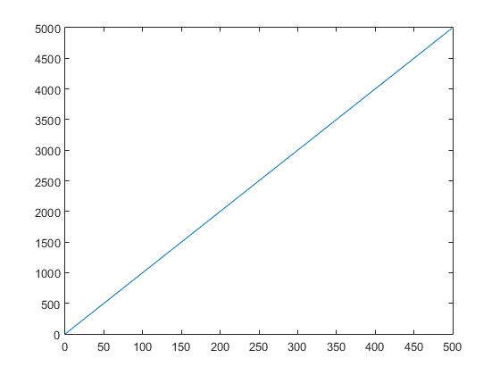
The above plot shows the best scenario, where we haven’t any noise effect, hence there’s no need of using a filter to smooth the signal.

But this isn’t the signal which we often encounter in the real world. In most applications, we have a noisy signal, i.e. one that was corrupted by noise.

In the following, it’s shown a MATLAB script that corrupts our previously defined time series with a normally distributed noise:

Such that:

An additive noise following a Gaussian distribution with zero-mean is of particular importance in the field of Digital Signal Processing (DSP), and it’s named Additive White Gaussian Noise (AWGN).

Figure 2 shows the plot of the noisy signal.

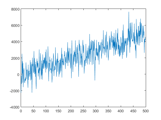
Now, it’s harder to assert about the trend, it seems that there’s a moderated growth, but there’s not a clear confirmation of this assumption, someone less careful can even say that the signal is simply floating around some straight line.

Is it the case? Let’s investigate it in more detail.

It’s common, but not necessarily required, to have a noise component of a very high frequency compared to the trend. In this way, we can achieve our objective of smoothing the signal by passing it through a low pass filter.

A low pass filter is a system which leaves the signal unchanged up to certain frequency:

Called the cut-off frequency, and suppresses the signal components whose frequencies are greater than the cut-off [2].

The simplest kind of low pass filter is called the ideal low pass filter, and it’s a system of frequency response defined by:

That is one for frequencies below:

And zero elsewhere, i.e. :

Although its simplicity, it happens that this kind of filter has some disadvantages, mainly due to its non-causal impulse response, which makes impossible implement a real-time filter.

Fortunately, many other simple filters can be adequately applied, and besides its easy implementation, they provide sufficient results for almost all situations. This is the case for investment analysis, where the investor is observing the asset price and trying to guess its trend over time.

One of the most used smoothing filters (low pass) is the Moving Average (MA) filter.

For example, in the above case of an investor trying to guess the asset’s trend, an MA filter is one of the favourite choices, due to its easy development and interpretation.

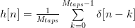
The MA causal impulse response:

For some defined number of taps:

It’s defined by:

This kind of filter is generally classified as Finite Impulse Response (FIR) filter.

We can interpret this filter as a system which adds the first:

values, and then divides the summation by:

That is, it computes the average.

After this, it replaces the oldest value for the most recent entry, then repeats the process of averaging. Therefore we have an average that is “running” through the time series, and at every step, it replaces the oldest value by the next one in the series.

One drawback of this filter is that it has a delay of:

Due to the need for accumulating them for the averaging process. Furthermore, its frequency characteristic is not so good in comparison with more complicated filters, but because of its straightforward implementation, it’s very used anyway.

Finally, the code snippet below shows the implementation of the MA filter.

Where the filtered signal is:

And it’s shown in Figure 3.

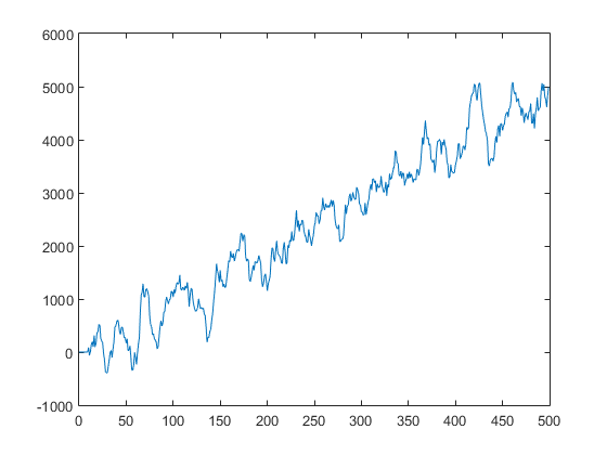
In this plot, we can see the delay effect previously described.

But more importantly, we can now make a more educated guess about the time series trend, which is growth, under the deterministic trend component shown in Figure 1.

Conclusion

In this article, we’d talked about some concepts related to signals and the problem of smoothing a time series corrupted by noise. Afterwards, we introduced the MA filter as a simple, yet useful, solution for noise filtering.

Finally, we developed an implementation of an MA filter in MATLAB and it’s replicated as a whole here:

References

[2] OPPENHEIM, A. V. and SCHAFER, R. W. Discrete-Time Signal Processing. 3E. Published By Pearson.

Originally published at https://medium.com/@rvarago